Tutorial Part I: Train Your First Model with YAPiC

Installation and Preparation of Training Data

Install YAPiC as explained here
The command line tool yapic should be available now:
```
yapic --help
```
Download and unzip leaf example data. It contains following files:
```
leaves_example_data/
├── leaf_labels_ilastik133.ilp
├── leaves_1.tif
├── leaves_2.tif
├── leaves_3.tif
├── leaves_4.tif
├── leaves_5.tif
├── leaves_6.tif
└── leaves_7.tif
```
The tif files are RGB images containing photographs of different leaf types.The images were saved with Fiji. Make sure to always convert your pixel images with Fiji. Large image series can be conveniently converted with Fiji by using batch processing.

The ilp file is a so called ilastik Project File and contains training labels. Next, we will have a look at the labels.
For looking at the label data, download and install Ilastik. We created the label data with Ilastik version 1.3.3.
Launch Ilastik and open the ilastik project leaf_labels_ilastik133.ilp

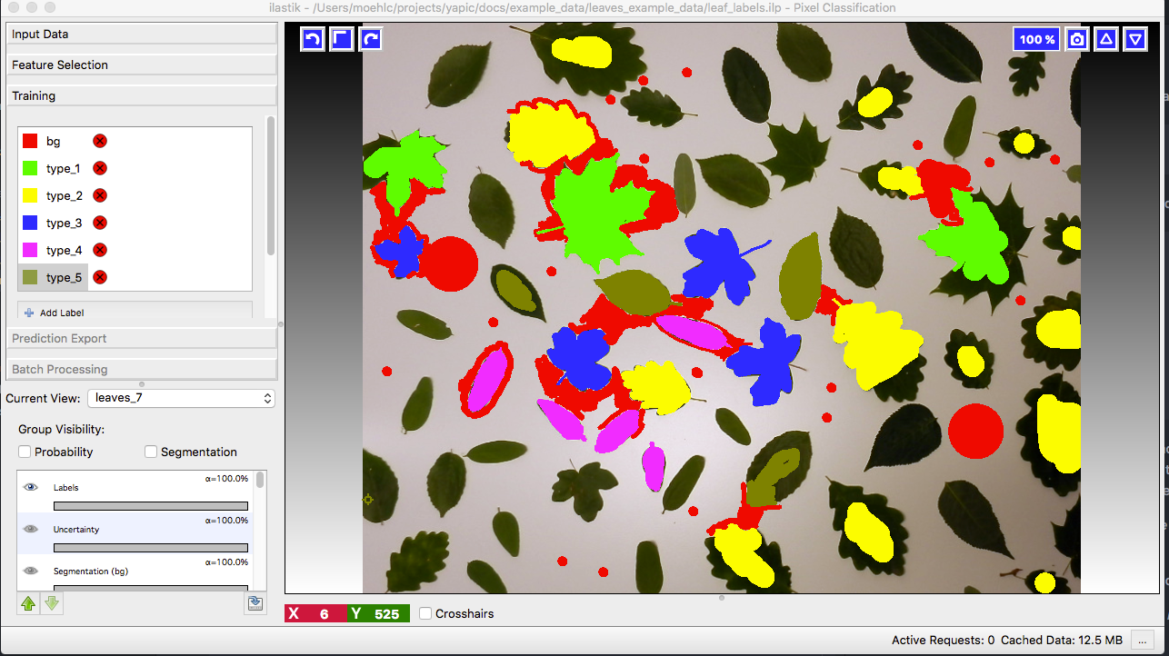
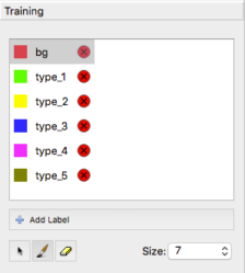
You see manually drawn labels for the leaves_7.tif image. There are labels for 6 different classes: 5 leaf types and the backgound class (red). In current view you can select one of the other images.

Ilastik comes with built in functionality for classifier training and pixel classification. It is very convenient to use and much faster than the deep-learing based classificaton of YAPiC. However this leaf classification task, can not be solved with Ilastik’s built in classification. For this reason, we use Ilastik in this case just as a tool for labeling and will train a classifier with YAPiC.
Add some more training data.

Choose some other images with less labels and use the brush to paint more image regions. The more labels you have, the better will be your training result. Amount of labels should be more or less balanced between all classes.
Save your updated Ilastik project: Project>>Save Project...

Model Training

Now you can start a training session with YAPiC command line tool:
```
yapic train unet_2d "path/to/leaves_example_data/*.tif" path/to/leaves_example_data/leaf_labels_ilastik133.ilp -e 800 --gpu=0
```
- unet_2d defines the type of deep learning model to train. We choose the original U-Net architecture as described in this paper.
- Next, we define the pixel data source with a wildcard. With wildcards you have to use quotation marks.
- Next, we have to define the label data source. In our case the ilastik project file path/to/leaves_example_data/leaf_labels.ilp
- The optional argument e defines the number of training epochs, i.e. the length of the training process.
- If you have multiple GPU cards available, you can select a specific GPU with the optional --gpu argument.
- Use yapic --help to get an overview about all arguments.

Training progress can be observed via command line output. Training 2500 epochs will take several hours.

Epoch 5/500
50/50 [==============================] - 63s 1s/step - loss: 1.7317 - accuracy:    5.3919 - val_loss: 1.6949 - val_accuracy: 3.7496
Epoch 6/500
50/50 [==============================] - 64s 1s/step - loss: 1.7241 - accuracy:    5.0915 - val_loss: 1.6836 - val_accuracy: 3.8097
Epoch 7/500
50/50 [==============================] - 64s 1s/step - loss: 1.7246 - accuracy:    5.4757 - val_loss: 1.6919 - val_accuracy: 3.6405
Epoch 8/500
17/50 [=========>....................] - ETA: 27s - loss: 1.7165 - accuracy:    5.5103

Training progress is also logged to loss.csv.
The best performing model (the model with the lowest validation loss) is repeatedly saved as model.h5.

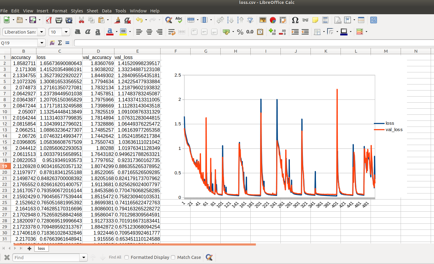
The loss of training data and validation data is continuously written to loss.csv file. You can open this file in any spreadsheet software (e.g. MS Excel) and plot loss and validation_loss: You see that the model initially learns to predict the data (the loss decreases). But from time to time, the curve falls back to a higher loss and training process starts again. You can also see, that training loss tends to be a bit lower than validation loss. The shape of the loss curve is very dependent on the dataset you process.

Please note that at the end of the 500 interations the validation loss is higher than some iterations earlier. YAPiC only stores the best performing model parameters, i.e. the model with lowest validation loss over the whole training period.

Apply your model

After the training process, the model.h5 file contains the best performing model, i.e. the model with best performance on the validation dataset. You have two options how to apply your model: Either you can run your model on a set of tif images by using YAPiC command line tool (the one you used for training) or you can export your model to run it in ImageJ/Fiji by using DeepimageJ plugin. We tested YAPiC trained models with DeepimageJ versions 1.0.1. and 1.2.0.

Apply model using YAPiC command line tool

Apply your model to the images

yapic predict model.h5 "path/to/leaves_example_data/*.tif" path/to/results

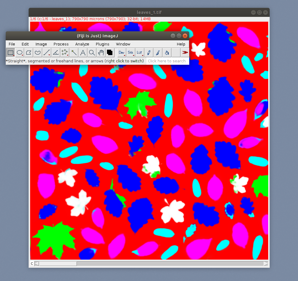
Predictions will be saved as 32 bit tif images in path/to/results.

You can open the result files in Fiji. Each channel represents one class (i.e. one of 5 leaf types or background).

Apply model in Fiji using DeepImageJ plugin

Go to part II for learning how to use you custom made leaf classifier in Fiji by using DeepImageJ plugin.